Storage Costs and Convenience Yield
Commodity futures prices don't exist in isolation from physical market realities. The relationship between spot and futures prices follows predictable economics based on storage costs, financing rates, and the value of holding physical inventory. Understanding this cost of carry model explains why futures curves take their shapes and helps identify when markets offer unusual opportunities.
The Cost of Carry Model
The theoretical relationship between spot and futures prices follows this formula:
F = S × e^(r + u - y)t
Where:
- F = Futures price
- S = Spot price
- r = Risk-free interest rate (annualized)
- u = Storage cost rate (annualized, as percentage of spot price)
- y = Convenience yield (annualized, as percentage of spot price)
- t = Time to expiration (in years)
- e = Euler's number (approximately 2.718)
For practical calculations, the simpler approximation works:
F ≈ S × (1 + r + u - y) × t
This formula states that futures prices should equal spot prices plus carrying costs (interest and storage) minus convenience yield.
Storage Cost Components
Physical commodities require infrastructure and capital to hold. These costs vary dramatically by commodity type.
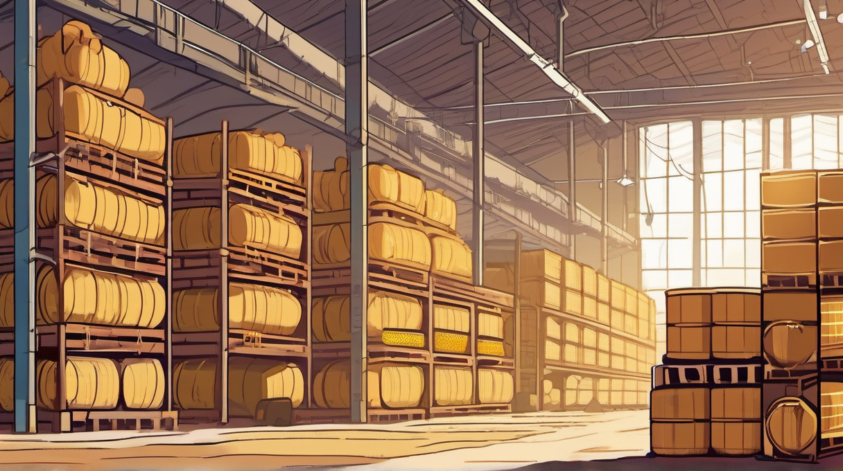
Warehousing
Crude oil: Onshore tank storage runs $0.25-$0.50 per barrel per month at Cushing, Oklahoma (the WTI delivery point). During the 2020 storage crisis, spot rates spiked to $1.00+ per barrel per month as available capacity disappeared.
Natural gas: Underground storage (depleted reservoirs, salt caverns) costs approximately $0.04-$0.08 per MMBtu per month. Working gas storage capacity in the U.S. totals approximately 4.7 trillion cubic feet.
Grains: Commercial grain elevator storage runs $0.03-$0.06 per bushel per month for corn and wheat. Quality degradation risk limits practical storage duration.
Metals: LME (London Metal Exchange) warehouse storage for copper and aluminum costs approximately $0.03-$0.05 per metric ton per day, plus loading/unloading fees of $15-$30 per ton.
Gold: Vault storage costs 0.1-0.3% of value annually at major custodians—substantially lower per-unit cost than industrial commodities because of gold's high value density.
Insurance
Insurance typically runs 0.1-0.3% of commodity value annually for most physical commodities. Oil and gas facilities carry higher rates due to fire and environmental liability risk. Precious metals in secure vaults have minimal insurance costs relative to value.
Financing
Holding physical inventory ties up capital. At current interest rates (4-5% for risk-free Treasury bills), financing costs represent a significant carrying cost component.
Example: Holding $1 million of physical copper for six months at 5% annual financing costs $25,000 in interest expense.
Total Storage Cost Examples
| Commodity | Monthly Storage | Annual Insurance | Financing (5%) | Total Annual Carry |
|---|---|---|---|---|
| Crude oil (per barrel) | $3.00-$6.00 | ~$0.20 | ~$3.75 | ~$7-$10 (9-13%) |
| Natural gas (per MMBtu) | $0.48-$0.96 | ~$0.05 | ~$0.15 | ~$0.70-$1.15 (20-35%) |
| Corn (per bushel) | $0.36-$0.72 | ~$0.02 | ~$0.22 | ~$0.60-$0.95 (13-20%) |
| Gold (per ounce) | ~$2-$6 | ~$2-$5 | ~$100 | ~$105-$110 (5-6%) |
Percentages based on approximate spot prices: oil $75/bbl, gas $3/MMBtu, corn $4.50/bu, gold $2,000/oz
Convenience Yield: The Value of Having Inventory
Convenience yield represents the benefit of holding physical commodity inventory rather than futures contracts. This benefit has real economic value in certain circumstances.
When Convenience Yield Is High
Supply disruptions: When pipeline outages, refinery fires, or port closures threaten supply, having physical inventory on hand allows continued operations. A manufacturer with copper stockpiles can keep producing while competitors scramble.
Production continuity: Refineries, smelters, and food processors face enormous costs from shutdowns. Keeping buffer inventory prevents expensive operational disruptions. The implicit value of this insurance is the convenience yield.
Quality or delivery concerns: Futures contracts deliver standardized specifications at designated locations. If you need specific grades or delivery to non-standard locations, holding physical inventory provides optionality that futures don't.
Seasonal demand: Heating oil distributors in the Northeast value inventory heading into winter. Agricultural processors value grain supplies during the gap between harvests.
Quantifying Convenience Yield
Convenience yield isn't directly observable—it's calculated as the residual that explains why futures trade below theoretical full-carry levels.
Calculation:
y = r + u - (F - S) / (S × t)
If the formula predicts futures should trade $5 above spot, but they actually trade $2 above spot, the $3 difference (annualized) represents convenience yield.
Typical convenience yields:
| Market Condition | Implied Convenience Yield |
|---|---|
| Well-supplied market | 0-2% annualized |
| Tight supply | 5-15% annualized |
| Supply crisis | 20%+ annualized |
Full Carry vs. Under Carry Markets
Full Carry
A market trades at "full carry" when futures prices equal spot plus total storage costs. This occurs when:
- Supply is abundant
- Storage is available and affordable
- No immediate need for physical delivery
- Convenience yield approaches zero
Example: Oil markets in late 2015-2016 traded at nearly full carry. Storage tanks filled as production exceeded demand. Contango spreads reached $0.60-$0.80 per barrel per month—almost exactly equal to financing and storage costs.
Implications: At full carry, physical arbitrage is marginally profitable. Traders buy spot crude, store it, and sell futures to lock in the carry spread. This activity puts a ceiling on how far into contango markets can trade.
Under Carry
A market trades "under carry" when futures prices fall below the full-carry theoretical price. This indicates positive convenience yield—the market values physical ownership.
Example: During the 2022 energy crisis, crude oil traded in steep backwardation. Six-month futures traded $10-$15 below spot prices despite financing and storage costs that should have pushed them above spot. The implied convenience yield exceeded 30% annualized.
Implications: Under-carry markets signal supply tightness. Producers and consumers who need physical supply bid up spot prices. Futures markets, reflecting expected normalization, trade at discounts.
Worked Example: Calculating Theoretical Futures Price
Given:
- Spot WTI crude oil: $75.00 per barrel
- Time to futures expiration: 3 months (0.25 years)
- Risk-free rate: 5.0% annually
- Storage costs: $0.40 per barrel per month = $4.80/year = 6.4% of spot
- Convenience yield: 2.0% annually (normal, well-supplied market)
Calculate theoretical 3-month futures price:
Using the approximation: F = S × [1 + (r + u - y) × t] F = $75.00 × [1 + (0.05 + 0.064 - 0.02) × 0.25] F = $75.00 × [1 + 0.094 × 0.25] F = $75.00 × [1 + 0.0235] F = $75.00 × 1.0235 F = $76.76
The theoretical 3-month futures price is $76.76, implying a contango spread of $1.76.
Scenario comparison:
| Scenario | Convenience Yield | 3-Month Futures | Spread |
|---|---|---|---|
| Normal supply | 2% | $76.76 | +$1.76 contango |
| Tight supply | 10% | $74.98 | -$0.02 backwardation |
| Supply crisis | 25% | $72.31 | -$2.69 backwardation |
Higher convenience yields push futures below spot, creating backwardation.
Practical Applications
Identifying Arbitrage Bounds
When futures exceed full-carry levels, physical arbitrage becomes profitable—buy spot, store, deliver against futures. This activity increases until the spread compresses.
When futures trade well below full-carry levels (high convenience yield), reverse arbitrage is theoretically possible—sell spot, buy futures, take delivery later. However, reverse arbitrage is difficult because finding commodities to borrow and sell short is often impractical.
Evaluating Storage Investments
Infrastructure investors evaluate storage facilities based on the spread between futures and spot. When contango spreads are wide, storage assets generate strong returns by capturing the time spread. When markets trade in backwardation, storage value diminishes.
Decision framework:
- Contango > storage costs: Storage profitable
- Contango < storage costs: Storage unprofitable
- Backwardation: Storage earns negative carry
Informing Hedging Decisions
Producers and consumers use cost of carry analysis to evaluate hedging economics:
- In backwardation: Producers can hedge at prices below current spot but lock in certainty
- In contango: Consumers can hedge at prices above current spot but may face immediate premium
Monitoring Checklist
For each commodity of interest:
- Calculate current spot-to-front-month spread
- Compare to estimated storage + financing costs
- Determine if market is full carry, under carry, or backwardation
- Monitor changes in spread as supply/demand shifts
Market indicators:
- Inventory reports (EIA weekly, USDA monthly)
- Storage capacity utilization data
- News on supply disruptions or logistics constraints
Understanding storage costs and convenience yield provides the foundation for interpreting futures curves. These concepts explain why crude oil can trade in backwardation during supply crises or deep contango during gluts—and what those curve shapes mean for investors and hedgers.
Related: Contango vs. Backwardation Explained | Commodity Index Construction | Hedging Programs for Producers and Consumers
Related Articles
Natural Gas Pricing Hubs and Seasonality
How natural gas pricing works across regional hubs, with seasonal patterns that create predictable price swings of $1-3/MMBtu between winter and summer.
Metals Markets: Precious vs. Industrial
The differences between precious metals (gold, silver, platinum) and industrial metals (copper, aluminum, zinc), with distinct demand drivers, trading venues, and price behaviors.
Building Regime Models for Portfolios
Learn to construct simple regime-based allocation models using trend, volatility, and macro indicators while avoiding common backtesting pitfalls.